The problem
Who plays like this player?
Imagine you want to find players who play similarly to a particular footballer.
How could a computer identify players with similar characteristics?
A player similarity experiment — and my favourite way to introduce traditional machine learning, because you can see exactly how the algorithm makes its decisions.
Imagine you want to find players who play similarly to a particular footballer.
How could a computer identify players with similar characteristics?
Use K-nearest neighbours (KNN) to compare players based on selected performance characteristics. Each player becomes a point in “feature space”, and the closest points are the most similar players.
| Player | Goals per game | Assists per game | Passes per game |
|---|---|---|---|
| Player A | 0.8 | 0.5 | 12 |
| Player B | 0.7 | 0.6 | 11 |
| Player C | 0.2 | 0.1 | 20 |
| Player D | 0.9 | 0.4 | 13 |
Player A, B and D look alike: lots of goals and assists, few passes. Player C is very different. KNN turns that intuition into maths.
Pick the stats that describe a player's style, like goals, assists and passes per game.
Treat each player as a point and measure the straight-line distance from your chosen player to every other player.
Sort by distance. The K nearest players — the “neighbours” — are the most similar.
Choose a player, the stats to compare and how many neighbours (K) to find. Then switch feature scaling off and watch the results change.
Distance is measured across all the features you've ticked — the chart shows two of them. Hover over a player for their stats.
| Player | Goals per game | Assists per game | Passes per game |
|---|---|---|---|
| Player A | 0.8 | 0.5 | 12 |
| Player B | 0.7 | 0.6 | 11 |
| Player C | 0.2 | 0.1 | 20 |
| Player D | 0.9 | 0.4 | 13 |
| Player E | 0.6 | 0.3 | 18 |
| Player F | 0.1 | 0.2 | 45 |
| Player G | 0.3 | 0.4 | 38 |
| Player H | 0.05 | 0.05 | 55 |
| Player I | 0.4 | 0.7 | 30 |
| Player J | 0.75 | 0.45 | 15 |
| Player K | 0.15 | 0.3 | 50 |
| Player L | 0.1 | 0.1 | 13 |
These are made-up example players for the demo. Players A–D match the example table above.
Goals, assists and passes are measured on very different ranges. Without scaling, the stat with the biggest numbers dominates the distance — and the “most similar” players are really just the players with a similar number of passes.
How far each stat spreads across the 12 example players:
A gap of 5 passes counts the same as a gap of 5 goals per game — which no player could ever have.
Min–max scaling squeezes every stat onto the same 0–1 range, so each one gets a fair say in the distance.
Try it in the demo: choose Player A and switch scaling off. Player L — who barely scores or assists — suddenly looks like one of the most similar players, just because their pass count is close.
KNN is one of the most intuitive ways to understand machine learning. There's no black box: you can see every point, every distance and exactly why the algorithm picked its answer. That makes it a great first step before more complex models.
This is a player similarity experiment, not a definitive scouting or recruitment model. Similarity depends heavily on which features you choose, how you scale them, and the context players perform in — their team, league and role.
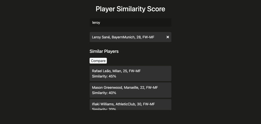
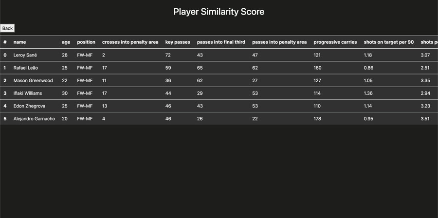
Search for a player and see who's most similar, then compare their stats side by side.